Measure developers should follow several steps when developing a risk adjustment or risk stratification model:

• Choose and define an outcome
• Define the conceptual model
• Identify potential data sources and variables
• Identify risk factors and timing
• Model and empirically test the data
• Assess the model
• Document the model

Some models may not lend themselves appropriately to all these steps, e.g., empirical testing. An experienced statistician and clinical expert together can help determine the need for each step.

Choose and Define an Outcome

When selecting outcomes appropriate for risk adjustment and/or stratification, the time interval for the outcome must be meaningful, the definition of the outcome must clearly define what to count and not to count, and one must be able to collect the outcome data reliably. An appropriate outcome has clinical or policy relevance. It should occur with sufficient frequency to enable statistical analysis unless the outcome is a preventable and serious health care error that should never happen. Measure developers should evaluate outcome measures for both validity and reliability, as described in the Blueprint Measure Testing content. Whenever possible, measure developers should consult with clinical experts, such as those participating in the technical expert panel (TEP), to help define appropriate and meaningful outcomes. Finally, as discussed in the supplemental material, Person and Family Engagement in Quality Measurement, patients should be involved in choosing which outcomes are appropriate for quality measurement. They are the ultimate experts on what is meaningful to their experience and what they value.

Define the Conceptual Model

Measure developers should develop a priori, a clinical hypothesis or conceptual model about how potential risk factors relate to the outcome. There is no one best way to model risk adjustment. The conceptual model serves as a map for development of a risk adjustment or stratification model. It defines the understanding of the relationships among the variables and, as such, helps identify which risk factors, patients, and outcomes are important, and which to exclude. Because the cost of developing a risk adjustment and/or stratification model may be prohibitive if the measure developer included every potential risk factor, the conceptual model also enables the measure developer to prioritize among risk factors and evaluate the cost and benefit of data collection. An in-depth literature review can greatly enhance this process. Alternatively, the existence of large databases and computational approaches such as machine learning allow for statistical analyses to explore the data for relationships between outcomes and potential, not yet clinically identified adjustment factors, but exist empirically. Measure developers should be aware of the potential for spurious relationships.

The first step in developing or selecting the conceptual model is identifying relationships among variables. This process should include

• Conducting a review of the literature and canvassing expert opinion to establish variable relationships and identify measurable patient factors related to the outcome and are either independent of the quality construct (i.e., for risk adjustment) or not independent (i.e., for stratification).
• Obtaining expert opinion from measured entities and subject matter experts with relevant specialties, experienced statisticians and research methodologists, and relevant interested parties such as patient advocates. Measure developers should use a TEP if seeking diverse input. The supplemental material, Technical Expert Panels, covers the standardized process for convening a TEP.
• Conducting empirical analyses to further support variable selection (when appropriate data are available) to identify potential factors for consideration by SMEs.

Identify the Risk Factors and Timing

Use a conceptual model and expertise promoting selection of these risk factors:

• Clinically relevant in the case of clinical risk factors
• Reliably collected
• Validly operationalized
• Sufficiently comprehensive
• Associated with the outcome
• Clearly defined
• Identified using appropriate time frames

In addition to these attributes, risk factors should also align with CMS CBE policies for endorsed quality measures if seeking CBE endorsement.

Acquire Data (Sample, if Necessary)

Health care data can come from many sources, but the three most frequently used are claims data, patient record data, and survey data. Of these, the most common source of data for developing risk adjustment models is claims data reported by the measured entity. However, identifying sources of social risk factors may be more difficult as measured entities historically have not collected or reported these data accurately or consistently. Once the measure developer identifies data sources and secures permission to use the data, they may need to link relevant databases and perform data preparation tasks, including assessment of data reliability and validity, if not previously confirmed. If using samples, the measure developer should draw the samples using predefined criteria and methodologically sound sampling techniques. The measure developer needs to use data from diverse measured entities and diverse patients. Testing to determine the suitability of data sources and testing for differences across data sources may also be necessary.

The alpha and beta testing discussion in the Measure Testing content provides details of testing processes.

Analyze the Data

In addition to clinical judgment used to define the conceptual model and select candidate variables, the measure developer should conduct empirical analysis to help determine which risk factors to include or exclude. While primarily used to assess addition of a biomarker to a risk model, measure developers may want to consider using net reclassification improvement (or index) techniques to compare risk models (e.g., Kerr et al., 2014; McKearnan et al., 2018). Measure developers should consider the four factors in the sections below when developing an appropriate risk adjustment model.

Sufficient Data

When creating a risk adjustment model, there should be enough data available to ensure a stable model. Different statistical rules apply to different types of models. For example, a model with a more common outcome may require more than 30 cases per patient factor to consistently return the same model statistics across samples. If the outcome is uncommon, then the number of cases required could be much larger (Iezzoni, 2013). Other factors may also affect the needed sample size, such as a lack of variability among risk factors with small sample resulting in partial collinearity among risk factors and a corresponding decrease in the stability of the parameter estimates. A statistician can provide guidance to determine the appropriate sample sizes based on the characteristics of the sample(s) and the requirements of the types of analyses in use.

Methods to Retain or Remove Risk Adjustors

Whenever possible, it is preferable to fit a model with as few variables as possible to explain any variance as completely as possible. This is often known as model simplicity or model parsimony. The principle of parsimony captures the balance between errors of underfitting and overfitting inherent in risk adjustment model development. For example, developing a model with many predictors can result in variables that primarily explain incremental variance unique to a data source or available samples (i.e., overfitting) and can also result in reduced stability of parameters due to increased multicollinearity (collinearity among more than two variables). In contrast, a model with fewer predictors may reduce the amount of explained variance possible for the quality measure (i.e., underfitting).

When evaluating these models, determination of the preferred model may depend on the availability of other samples to validate findings and detect overfitting and the degree of multicollinearity among predictors. However, in general, the simpler model may provide a more robust explanation since it uses fewer variables to explain nearly the same observed variability. In addition, simpler models are likely to reduce the cost of model development because the simpler models involve collecting fewer variables and may be less likely to show signs of model overfitting. Measure developers may achieve parsimonious models by omitting statistically significant predictors offering minimal improvement in predictive validity or overall model fit and by combining clinically similar conditions to improve performance of the model across time and populations. However, in situations with high visibility or potentially widespread fiscal repercussions, CMS has employed some of the most sophisticated models available, such as Hierarchical Generalized Linear Models as described in Statistical Issues in Assessing Hospital Performance.

When developing a risk adjustment model, the choice of variables for inclusion often depends on estimated parameters in the sample rather than the true value of the parameter in the population. Consequently, when selecting variables to retain or exclude from a model, the idiosyncrasies of the sample, as well as factors such as the number of candidate variables and correlations among the candidate variables, may determine the final risk adjustors retained in a model. Improper model selection or not accounting for the number of, or correlation among, the candidate variables may lead to risk adjustment models that include suboptimal parameters or overestimated parameters—making them too extreme or inappropriate for application to future datasets. This is model overfitting, as the model is more complicated than needed and describes random error instead of an underlying relationship.

The measure developer can use statistical model fitting methods such as stepwise regression, or an adaptation thereof, to identify the simplest combination of variables providing high predictive value without overfitting. Another step to consider to minimize model overfitting is selection of model variables based on resampling methods and assessment of the model in multiple/diverse samples (refer also to the section below on Generalizability). There is a strong recommendation to consult with clinical experts, ideally during candidate variable selection, when examining the performance of candidate variables in risk adjustment models. This expertise may help inform relationships among model parameters and may help justify decisions to retain or remove variables.

Generalizability

Measure developers should take steps to ensure generalizability of their findings to target populations when developing their models. Measure developers should begin with parameter estimation and test with diverse measured entities and persons. Researchers often use two datasets in building risk adjustment models: a development (i.e., calibration) dataset and a validation dataset. Measure developers should use the development/calibration dataset to develop the model or calibrate coefficients, and use the validation dataset to determine the appropriate extent of the application of the model to parent populations. When assessing generalizability to the population of the development dataset, the measure developer may collect the two datasets independently—which can be costly—or the measure developer may split one dataset using random selection.
Either of these methods enables evaluation of the model’s generalizability to the population and helps avoid any model features arising from idiosyncrasies in the development sample. Additional validation using samples from different time periods may also be desirable to examine stability of the model over time.

Multilevel (Hierarchical) Data

The potential for observations to be “nested” within larger random groupings or levels frequently occurs in health care measurement (e.g., there is nesting of patients under physician groups, which may in turn be nested under hospitals). The risk adjustment model should account for these multilevel relationships when present. In developing risk adjustment models, measure developers should investigate theoretical and empirical evidence for potential patterns of correlation in multi-level data. For example, the risk adjustment model should address patients in the same Inpatient Rehabilitation Facility (IRF) with tendencies to have similar outcomes based on a variety of factors.

The measure developer should examine these multilevel relationships by building models designed to account for relationships between observations within larger groups. Terms for these types of models include multilevel model, hierarchical model, random-effects model, random coefficient model, and mixed model. These terms all refer to models explicitly modeling the “random” and “fixed” variables at each level of the data. In this terminology, the assumption is to measure a “fixed” variable without error, where the value or measured characteristic is the same across samples (e.g., male vs. female, nonprofit vs. for-profit facility) and studies. In contrast, the assumption is “random” variables are to be values drawn from a larger population of values (e.g., a sample of IRFs), where the value of the random variable represents a random sample of all possible values of that variable.

Traditional statistical methods (i.e., linear regression and logistic regression) require observations (e.g., patients) in the same grouping to be independent. When observations co-vary based on the organization of larger groupings, these methods fail to account for the hierarchical structure and there are violations of the assumptions of independence among the observations. This situation may ultimately lead to underestimated standard errors and incorrect inferences. Attempts to compensate for this problem by treating the grouping units as fixed variables within a traditional regression framework is undesirable because it reduces the generalizability of the findings.

Multilevel models overcome these issues by explicitly modeling the grouping structure and by assuming the groups reflect random variables (usually with a normal distribution) sampled from a larger population. They consider variation at different grouping levels and allow modeling of hypothesized factors at these different levels. For example, a multilevel model may allow modeling patient-level risk factors along with the facility-level factors. If the measure developer has reason to suspect hierarchical structure in the measurement data, they should examine these models. The measure developer should apply the models within common frameworks used for risk adjustment (e.g., ordinary least squares regression for continuous outcomes, logistic regression for binary outcomes), as well as less common longitudinal frameworks such as growth (i.e., change) modeling.

Developments in statistics are enabling researchers to improve both the accuracy and the precision of nested models using computer-intensive programs. These models include estimation of clustering effects independent of the main effects of the model to better evaluate the outcome of interest. For example, there are indications use of precision-weighted empirical Bayesian estimation produces more accurately generalizable coefficients across populations than methods relying on the normal curve for estimation (e.g., linear regression). There is also use of hierarchical factor analysis and structural equation modeling.

Assess the Model

There is a requirement to assess the model for a newly developed risk adjustment model and when using an “off-the-shelf” adjustment model because an existing risk adjustment model may perform differently in the new quality measure context. When multiple data sources are available (e.g., claims and chart-based data), the recommendation is to assess the model performance for each data source to allow judgment regarding the adequacy and comparability of the model across the data sources.
Measure developers should assess all models they develop to ensure the models do not violate underlying assumptions (e.g., independence of observations or assumptions about underlying distributions) beyond the robustness established in the literature for those assumptions. Measure developers should assess models to determine predictive ability, discriminant ability, and overall fit of the model.

Some examples of common statistics used in assessing risk adjustment models include the R2 statistic, receiver-operating characteristic (ROC) curve, the Akaike Information Criterion (AIC) or the Bayesian Information Criterion (BIC), and Hosmer-Lemeshow test (HL test). However, several other statistical techniques can enable measure developers to assess different aspects of model fit for different subpopulations as well as for the overall population. The engagement of an experienced statistician is critical to ensure the selection of the most appropriate methods during model development and testing.

• R2 Statistic - A comparison of the R2 statistic with and without selected risk adjustment is frequently used to assess the degree to which specific risk-adjusted models predict, explain, or reduce variation in outcomes unrelated to an outcome of interest. Measure developers may use the statistic to assess the predictive power of risk-adjusted models overall. In that case, values for R2 describe how well the model predicts the outcome based on values of the included risk factors.

  The R2 value for a model can vary, and no firm standard exists for the optimal expected value. Experience or previously developed models may inform which R2 value is most reasonable. In general, the larger the R2 value, the better the model. However, the measure developer may also need clinical expertise to help assess whether remaining variation is primarily related to differences in the measured quality. Extremely high R2 values can indicate something is wrong with the model.

• ROC Curve, Area Under the Curve (AUC), and C-statistic - Measure developers often use the ROC curve to assess models predicting a binary outcome (e.g., a logistic regression model), where there are two categories of responses. Measure developers may plot the ROC curve as the proportion of target outcomes correctly predicted (i.e., a true positive) against the proportion of outcomes incorrectly predicted (i.e., a false positive). The curve depicts the tradeoff between the model’s sensitivity and specificity.

  Figure 1 shows an example of ROC curves. Curves approaching the 45-degree diagonal of the graph represent less desirable models (Curve A) when compared to curves falling to the left of this diagonal indicating higher overall accuracy of the model (Curves B and C). A test with nearly perfect discrimination will show a ROC curve passing through the upper-left corner of the graph, where sensitivity equals 1, and 1 minus specificity equals zero (Curve D).

  The ROC AUC often quantifies the power of a model to correctly classify outcomes into two categories (i.e., discriminate). The AUC, sometimes referred to as the c-statistic, is a value varying from 0.5 (i.e., discriminating power not better than chance) to 1.0 (i.e., perfect discriminating power). The interpretation of the AUC can represent the percent of all possible pairs of observed outcomes in which the model assigns a higher probability to a correctly classified observation than to an incorrect observation. Most statistical software packages compute the probability of observing the model AUC found in the sample when the population AUC equals 0.5 (i.e., the null hypothesis). Both non- parametric and parametric methods exist for calculating the AUC, and this varies by statistical software.

Image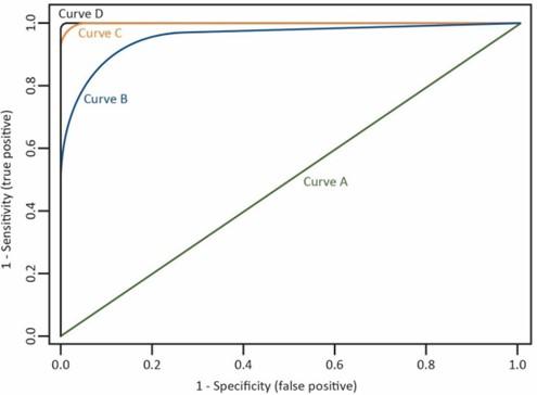

Figure 1. Example of ROC Curves

The Akaike Information Criterion (AIC) and the Bayesian Information Criterion (BIC) – The measure developer can use AIC and BIC to compare different logistic or linear regression models created from the same set of observations. Calculation of both the AIC and BIC is from the likelihood, a measure of the fit of the model. With the introduction of additional variables, the likelihood of a model can only increase, but both the AIC and BIC contain a penalty for the number of variables in the model. This means an additional variable must explain enough extra variation to “make up for” the additional complexity in the model. The measure developer calculates AIC and BIC as (where k is the number of variables in the model and n is the number of observations in the model):

AIC = -2*log (maximum likelihood) + 2*k 

BIC = -2*log(likelihood) + k*ln(n)

The magnitude of the BIC penalty depends on the total number of observations in the dataset (the penalty is higher for a larger dataset), but the penalty for the AIC is the same regardless of the dataset size. A higher likelihood represents a better fit, because the measure developer calculates the AIC and BIC from -2*log(likelihood), lower values of AIC and BIC represent better models (Akaike, 1974; Schwarz, 1978).

• The Hosmer-Lemeshow (HL) Test - Although the AUC/c-statistic values provide a method to assess a model’s discrimination, the measure developer can assess the quality of a model by how closely the predicted probabilities of the model agree with the actual outcome (i.e., whether predicted probabilities are too high or too low relative to true population values). This is known as calibration of a model. The HL test is a commonly used procedure for assessing the calibration of a model and the goodness of fit in logistic regression in the evaluation of risk adjustment models. This test assesses the extent to which the observed values/occurrences match expected event rates in subgroups of the model population. However, as with any statistical test, the power increases with sample size. This can be undesirable for goodness of fit tests because in very large data sets, there is significance in small departures from the proposed model. Meaning, statistically, the measure developer may deem the goodness of fit poor, even though the clinical significance is small to none. An alternative to consider is the dependence of power on the number of groups (e.g., deciles) used in the HL test. Using this approach, the measure developer can standardize the power across different sample sizes in a wide range of models. This allows an "apples-to-apples" comparison of goodness of fit between quality measures with large and small denominators (Paul, et al., 2012).

Generally, in a well calibrated model, the expected and observed values agree for any reasonable grouping of the observations. Yet, high-risk and low-frequency situations pose special problems for these types of comparison methodologies; therefore, an experienced statistician should address such cases.

The expectation is the measure development team will include a statistician to accurately assess the appropriateness of a risk-adjusted model. Determining the best risk-adjusted model may involve multiple statistical tests more complex than those cited here. For example, a risk adjustment model may discriminate very well based on the c-statistic, but poorly calibrated. Such a model may predict well at low ranges of outcome risk for patients with a certain set of characteristics (e.g., the model produces an outcome risk of 0.2 when roughly 20% of the patients with these characteristics exhibit the outcome in population) but predict poorly at higher ranges of risk (e.g., the model produces an outcome risk of 0.9 for patients with a different pattern of characteristics when only 55% of patients with these characteristics show the outcome in population). In this case, the measure developer should consult one or more goodness-of-fit indices to identify a superior model. Careful analysis of different subgroups in the sample may help to further refine the model. This may require additional steps to correct bias in estimators, improve confidence intervals, and assess any violation of model assumptions. Moreover, differences across groups for non-risk-adjusted measures may be clinically inconsequential when compared to risk-adjusted outcomes. It may be useful to consult clinical experts in the subject matter to provide an assessment of both the risk adjustors and utility of the outcomes.

Document the Model

The documentation ensures relevant information about the development and limitations of the risk adjustment model are available for review by consumers, purchasers, and measured entities. The documentation also enables these parties to access information about the factors incorporated into the model, the method of model development, and the significance of the factors used in the model.

Typically, the documentation contains

• Identification or review of the need for risk adjustment of the quality measure(s).
• A description of the sample(s) used to develop the model, including criteria used to select the sample and/or number of sites/groups, if applicable.
• A description of the methodologies and steps used in the development of the model or a description of the selection of an off-the-shelf model.
• A listing of all variables considered and retained for the model, the contribution of each retained variable to the model’s explanatory power, and a description of how the measure developer collected each variable (e.g., data source, time frames for collection).
• A description of the model’s performance, including any statistical techniques used to evaluate
• performance and a summary of model discrimination and calibration in one or more samples.
• Delineation of important limitations such as the probable frequency and influence of misclassification when the model is used (e.g., classifying a high-outcome measured entity as a low one or the reverse) (Austin, 2008).
• Enough summary information about the comparison between unadjusted and adjusted
• outcomes to evaluate whether the model’s influence is clinically significant.
• A section discussing a recalibration schedule for the model to accommodate changes in medicine and in populations; the first assignment of such a schedule is normally based on the experience of clinicians and the literature’s results and then later updated as needed.

The measure developer should fully disclose all quality measure specifications, including the risk adjustment methodology. The Measure Information and Justification Form (MIJF) & Instructions and Measure Evaluation Report and Instructions, all found in Templates, provide guidance for documenting the risk adjustment information.

If not modeled in the CQL, the measure developer should provide the risk adjustment instructions in the HQMF and human-readable HyperText Markup Language identifying where the user may obtain the complete risk adjustment methodology.
If calculation requires frequently changing, database-dependent coefficients, the measure developer should disclose the existence of these coefficients and the general frequency with which they change, but they do not need to disclose the precise numerical values assigned, as they vary over time.

Key Points

Risk adjustment is a method measure developers can use to account for confounding factors when calculating performance scores. Risk adjustment is especially important in the context of CMS programs using performance scores as a basis for calculating the amount of incentives or penalties for value-based purchasing and many APMs. As such, measure developers should evaluate the need for risk adjustment, stratification, or both, for all potential outcome measures and statistically assess the adequacy of any strategies they use. Measure developers should also consider the appropriateness of adjusting for social risk (i.e., socioeconomic factors) for these quality measures. Measure developers must determine on a case-by-case basis whether they should adjust a quality measure for social risk.
When developing a risk adjustment model, measure developers must identify and clearly define a sample to test the model. That sample should consist of high quality (i.e., valid, reliable, and comprehensive) data, with appropriate time intervals for all model variables. Further, measure developers should provide evidence all variables included in the model are clinically meaningful. Measure developers should also consult with an experienced statistician to outline a sound analytic, scientifically rigorous and defensible approach —including information about how to assess the model (e.g., the R2 statistic, ROC curve, and HL test). Finally, measure developers should document information about the development and limitations of the risk adjustment model to ensure interested parties can appropriately review and interpret quality measure scores.